The Journey of Global Liquidity

• Tracking global liquidity is essential because it influences all assets. Liquidity flows from central banks, governments, and regulations through the economy down to markets, shaped by risk-perception, spending, asset purchases, and levered by credit.

• Because liquidity is driven by multiple evolving factors, modelling it helps reduce subjective bias. Besides, upstream liquidity doesn’t spread evenly downstream, leading to an uneven concentration of risks. 

• Liquidity also transmits with varying delays, offering both forward-looking signals and backward-looking explanations. Given the role of investor psychology, behavioural understanding is necessary.

• Tracking liquidity is a continuous process that must adapt to the increasing complexity of the financial system and the changing nature of shocks.

• Importantly, assets behave asymmetrically across liquidity regimes. Liquidity risk is also convex - meaning there is a ‘cliff effect’ when liquidity dries up – and assets themselves have nonlinear sensitivity to liquidity. Understanding these convexities is critical.

• Finally, liquidity sets the tone for markets, which helps stay level-headedness during periods of stress.

• Today, global liquidity is generally benign but imbalanced, as market liquidity overstates its true abundance. That imbalance reflects the current paradox of short-term tailwinds co-existing with multiple longer-term tail-risks. While this supports asset prices, it also leaves them vulnerable to minor shocks, atypical chain reactions, more hawkish monetary bias, and a gradual erosion of credit conditions. 

• In particular, the growing complexity in money-market plumbing is adding vulnerability. The US Federal Reserve’s balance sheet holds a prominent role in determining liquidity, which is managed by altering the level of its assets, held primarily in Treasuries and MBS. On December 12th, the Fed started its Reserve Management Purchases (RMP) program to ensure reserves operate in an ample regime, which allows banks to provide adequate market liquidity. Although not being a proper QE, RMP expands the Fed’s balance sheet adding liquidity at macro level.

• Moreover, the liquidity regime has shifted in recent years, experiencing more frequent shocks than during the “great moderation” of the previous decade. Unlike in the past, when economic dynamics were the primary drivers, these shocks are emerging from a broader set of influences and rippling through a more complex financial system, making them harder to predict. Looking to the future, we expect this more volatile liquidity regime to persist.

• It is thus essential to factor liquidity into portfolio construction. Alongside growth and inflation, liquidity explains more than half of the performance of risky assets and cannot be overlooked. Liquidity also warned of 2/3 of significant equity drops over the past 30 years, albeit with varying notice periods. 

• Understanding the current liquidity regime helps define broad risk levels, while the near-term liquidity environment guides tactical adjustments. Assessing how assets react to liquidity, and the current intensity of its influence helps fine-tune portfolio positioning – especially today, when diversified allocations show heightened sensitivity to liquidity changes. Furthermore, understanding liquidity’s impact on the market structure, volatility, correlations, and alpha generation, enhances risk management.

Liquidity runs from the macro level down to the markets, back and forth

Tracking global liquidity is essential because it influences all assets, which has significant implications for portfolio construction. However, analysing global liquidity is complex: while measuring the initial supply is relatively straightforward, understanding how it spreads and multiplies is challenging.

The upstream supply of liquidity originates from central banks, fiscal policies and, to some extent, regulations. When economic growth slows while inflation and market expansion remain reasonable, liquidity is typically increased, and vice versa.

Liquidity then spreads to the rest of the economy down to markets, function of the perception of risk, through spending, asset purchases, and levered by credit. In times of high uncertainty or risk perception, liquidity tends to remain in savings and cash, with limited leverage. Conversely, when liquidity is abundant, economic agents are more inclined to take on additional risk.

Assessing downstream liquidity is complicated due to the variety of liquidity channels and economic agents, each exhibiting diverse behaviours and facing specific circumstances.

While macro factors strongly influence market liquidity, market events, conversely, also impact macro trends through various channels. For example, a rising perception of risk among investors often spreads to other economic agents. Additionally, significant changes in market prices create wealth effects that can alter corporate or household spending patterns.

How our Global Liquidity Barometer is constructed

Our Global Liquidity Barometer monitors this liquidity journey. At the Macro level, the analysis begins upstream with the supply of liquidity, a critical component. For instance, we analyse the various monetary levers and whether they are restrictive or accommodative. Liquidity then flows from one balance-sheet to another, forming the available pool for economic agents. Once on their balance sheets, we track how liquidity continues to circulate based on how these agents utilise it. In particular, we look at the nature of their income and spending and whether they use leverage. 

The transmission of liquidity can be amplified by foreign flows, so understanding the wealth creation abroad and the recycling of savings matters. Banks also play a crucial role in this process, particularly in Europe. Flows from derivatives, private assets, and cryptocurrencies increasingly matter too. At the intersection of liquidity and market dynamics, investors’ trading behaviour offers valuable insights into liquidity, such as the level of cash in traders’ accounts, the intensity of short selling, or brokers’ funding costs. Furthermore, two macro components influence all economic agents: the perceived intensity of risk and actual liquidity events. 

Finally, we monitor potential liquidity risks among smaller economic agents, focusing on those arising from liquidity mismatches, over-leverage, excessive risk concentration, and contagion risk – such as the interconnections between banks and non-bank financial institutions. This section of our Barometer is not intended to be exhaustive; rather, it is gradually expanded as the financial system grows more complex.

We refer to the above analyses as ‘Macro Liquidity’. We then monitor liquidity at a Market level (‘Market Liquidity’). Financial conditions can help identify market liquidity stress early on. Our in-house indicators allow us to have a critical view of the various indicators available in the market. These are intentionally designed to be simple, making them very practical. While ours require more maintenance, they seek to offer a more holistic view. 

Additionally, we examine a variety of trading patterns. As there is no straightforward way to quantify liquidity in dollar terms at the market level, instead, we track the smoking gun evidence of its various effects. To that aim, we first look at trading stability through the lenses of more than 50 signals that are indicative of stress, both at the security and index levels. Second, anomalies and shifts in asset relationships across market segments can also reveal liquidity imbalances, among other factors.  

We gauge the level of stress in a variety of assets most sensitive to liquidity in each key market segments – including securitised assets, deep credit markets, vulnerable areas in equities etc. – which may be symptomatic of stress. 

Market flows provide complementary insights into market liquidity, in particular their volatility and specific asset movements from origin to destination.

Finally, we track signs of contagion across the above liquidity factors, which may amplify and precipitate trends in liquidity. We assign an exponential weight to this contagion factor. 

The charts below display our Global Liquidity Barometer, which combines both Macro and Market Liquidity.

 

1. Liquidity is a pendulum always on the move, which rarely finds a perfect balance

Global liquidity constantly fluctuates due to lags in response to macro changes. It also tends to be mean-reverting: when macro conditions weaken, liquidity is typically added, and vice versa. Excessively abundant or scarce liquidity usually signals an upcoming turning point, often influenced by changes in authorities’ support. 

True equilibrium in global liquidity is rare for several reasons. First, liquidity data are inherently incomplete, as liquidity is the sum of multiple moving parts. Second, identifying the equilibrium liquidity level is as much an art as a science and is often recognised only in hindsight. Third, liquidity is influenced by subjective perceptions of risk, which can vary widely. Finally, the economy is frequently hit by shocks of different kinds, making the real impact on liquidity difficult to assess in real-time.

Because of these complexities, without a holistic and model-driven approach to monitoring global liquidity, investors risk overreacting – either succumbing to panic or developing a false sense of security.
 

2. Upstream liquidity doesn’t spread out evenly downstream

Macro Liquidity, supplied upstream, does not evenly distribute downstream. Differences in regulatory environments, fiscal incentives or repressions, the creditworthiness of borrowers, market access and infrastructure can impede the smooth transmission of liquidity. For example, liquidity mismatches in US regional banks and their concentrated exposures to commercial real estate have limited the local flow of capital.

Additionally, liquidity is not always deployed efficiently. Factors, including geopolitics, investor psychology (driven by fear and greed), and government interventionism, can lead to misallocations of capital. During periods of excess liquidity, this can fuel speculative bubbles or selloffs regardless of the overall liquidity and fundamentals. 

Similarly, liquidity does not spread out evenly across regions and across assets, and is influenced by relative profitability, growth prospects, and risk perceptions. Spotting these divergences may help refine allocation decisions.

 

3. Liquidity spreads with varying delays, carrying both lagging and leading signals 

Liquidity passes through different transmission channels at varying speeds. For example, changes in central banks’ balance sheets typically take 6 to 12 months to influence M2 aggregates, which then impact markets within up to 3 months. Fiscal transfers tend to have a more indirect impact, except when they are massive and/or directly targeting liquidity at end-users (during Covid-19, for example).

Moreover, liquidity factors differ in their persistence: commodity-driven inflation usually affects prices within 6 weeks and is quickly absorbed, whereas service-driven inflation tends to have a longer-lasting impact, which matters for monetary policies.

Modelling these leading, coincident, and lagging effects helps to anticipate the dynamics of global liquidity to some extent.

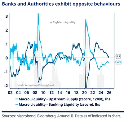
In this regard, the liquidity relay from the banking sector is noteworthy, as most credit - particularly in Europe- is channelled this way. Banks tend to be highly reactive – they quickly tighten lending when conditions deteriorate but are equally swift to increase risk-taking when conditions improve. Consequently, their behaviour often contrasts with that of authorities, who typically inject liquidity precisely when market conditions worsen.

 

 

4. The evolving nature of shocks and their impact on liquidity reveal new mechanisms 

Tracking liquidity is a constant work-in-progress. Shocks reveal new mechanisms and rarely cause stress in the same way as the last. Moreover, as the financial system grows more complex, new developments must be monitored – such as the rise of non-bank financial intermediation, decentralised finance, digital payments including digital currencies, the liquidity effects of systematic trading, increased retail participation, and unconventional deficit funding.

Unusual economic agents’ reaction to changes in liquidity can signal the influence of these emerging factors. Therefore, paying attention to the details is just as important as grasping the overall picture.

 

5. Tracking liquidity involves behavioral finance

Global liquidity is shaped by both supply and demand dynamics, as well as the emotional forces of fear and greed. Investor behaviour plays a key role: optimism boosts demand and liquidity, while fear can quickly dry it up. Herding and risk perception amplify these effects, causing liquidity to swing sharply, as illustrated in the chart that shows how the FOMO factor (the “Fear of Missing Out”) interplays with liquidity. In short, global liquidity reflects not only economic fundamentals but also the collective psychology of market participants.

 

 

6. Assets’ sensitivity to liquidity is not linear

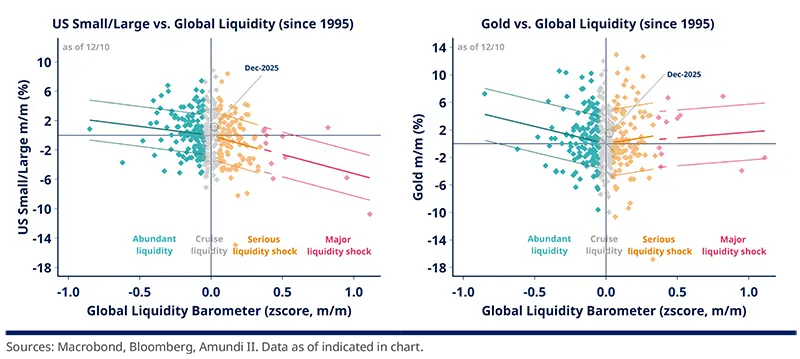
Assets naturally respond differently to a given liquidity environment. However, three important factors are often overlooked: first, liquidity risk is convex, meaning liquidity may experience a “cliff effect” as it dries out; second, assets themselves usually face changing sensitivities as liquidity tightens (or expands), which may disproportionately impact their returns; third, assets display asymmetric behaviour depending on the liquidity regime. For instance, the charts below show that US Small Caps are more severely impacted by higher liquidity stress (orange and red dots) than they benefit when liquidity improves (green dots). In contrast, gold responds positively to liquidity shocks.

By modelling global liquidity and stress-testing asset reactions, we can better understand these non-linear behaviours and more effectively manage asymmetric risks. We elaborate on this matter in a later section.

Small Cap: unfavourable risk symmetry to Liquidity Gold: favourable risk symmetry to Liquidity

 

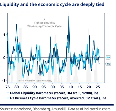
7. Liquidity is tightly linked to the economic and credit cycles and sets the tone for markets

The economic cycle reflects the dynamic interactions between households, corporates, the government, and the foreign sector, where one agent’s spending and borrowing is someone else’s income and lending. The exchange of goods and services among these economic agents generates circular money flows, which authorities attempt to smooth through monetary, fiscal and regulatory measures. The volume of these money flows forms the foundation of global liquidity.

In other words, global liquidity is closely linked to both the economic and credit cycles in a mutual interplay, and can be thought of as the “fluidity” of the cycle itself.

As a result, the analysis of liquidity can help define which phase of an economic cycle we’re in.

 

 

It also implies that fluctuations in global liquidity set the overall tone for markets. When liquidity is abundant, shocks, stresses, market frictions, and doubts tend to have manageable, localised, and short-lived impacts. Conversely, when liquidity is scarce, these same events can trigger outsized, spiralling effects across markets.

Therefore, tracking liquidity provides valuable insight about how to respond to shocks. Abundant liquidity should, as a general principle, generally encourage investor optimism, audacity and buy-on-dip strategies, while scarce liquidity should call for caution and avoiding attempts to catch falling knives.
 

8. Keeping track of liquidity helps stay level-headed when stress hits 

A holistic, model-driven approach helps reduce subjective biases, helping to prevent overreactions or denial – especially during periods of liquidity stress.

When a liquidity event occurs, it also helps to better assess its root causes (whether cyclical, structural, or driven by risk-perception), as this can be crucial to determining its likely severity.
 

9. There is a high barrier to tracking liquidity 

Monitoring liquidity can feel as daunting as trying to put the world into an equation. 

It involves extensive data crunching, especially when examining liquidity at the level of single securities. A dedicated team of data scientists at Amundi seeks to capture micro liquidity signals.

This process also demands substantial preliminary modelling. For example, while uncertainty clearly affects liquidity, its vague nature makes it difficult to measure directly, requiring dedicated models. Similarly, the impact of systematic trading – where flows are often opaque – requires specific indicators to detect signs of systematic activity.

The current state of global liquidity

After experiencing extreme stress in 2022, global liquidity has since reverted to a more stable state, though punctuated by milder yet noticeable shocks. These include stress in 2023 caused by liquidity mismatches in a few US banks that led to the demise of Credit Suisse, followed by the 2024 summer stress caused by unwinding carry trades and JPY volatility, and the still fresh, high turbulences in the Spring of 2025.

The liquidity stress in Spring 2025 was largely driven by a surge in risk perception amid a roaring trade war, a rapid series of policy shifts in the US, concerns about Developed Markets public deficits and fears of fast-paced dollar debasement. This led to a surging stress in market liquidity, amplified by a contagion effect.

While intense, the episode was short-lived as i) risk-perception rapidly receded (the pace of policy changes in the US moderated and fears of a major disruption in global capital flows dissipated); ii) economic agents’ behaviour remained largely unchanged; and iii) authorities gradually started to lift their still restrictive stance.

 

Currently, global liquidity is reasonably abundant, driven by a lower risk-perception, some monetary easing and deregulation, and anchored by moderate corporate and household credit, which both have room to lever up. 

However, this liquidity is imbalanced as most of the abundance comes from market liquidity and easing risk-perception, whereas macro liquidity remains around trend. Liquidity actually mirrors today’s paradox: short-term tailwinds co-exist with multiple longer-term tail risks – including tech disruption and profitability concerns, potential geopolitical escalations, rising debt and deficits, shifts in the global order and dollar‑debasement risk, and the ticking bomb of inequality. High trading liquidity therefore sits alongside caution by many economic agents. That imbalance means even minor shocks could quickly temper market optimism. The sheer variety of longer‑term risks also raises the odds that liquidity gets hit by an atypical combination of events.

Additionally, while liquidity is not at the excesses that might prompt authorities to pull back, it is moving closer to that threshold.

Furthermore, credit markets are likely entering a mid-cycle phase, with bottoming spreads and a slow fundamental deterioration – which would reverberate through liquidity.

Finally, money‑market plumbing is becoming more complex, adding further vulnerabilities (see the Focus on the next page, which elaborates on the Fed’s recent operations).

Overall, global liquidity is benign and backed by fundamentals, but market liquidity is overstating its abundance. As a result, the environment remains favourable for assets today, yet vulnerable to minor shocks, unusual chain reactions, more hawkish monetary bias, and a gradual erosion of credit conditions.

Global Liquidity outlook

Putting it in perspective, the liquidity regime appears to have shifted, becoming more volatile with more frequent shocks compared to the “great moderation” of the previous decade. By then, liquidity was unusually abundant, supported by low interest rates, quantitative easing, fiscal stimulus, and stabilised by tighter financial regulations.

In the current decade, liquidity is structurally less abundant, amid normalising monetary accommodation, growing fiscal constraints, and unsettled by a series of disruptive shocks.

While liquidity swings and shocks are not necessarily larger than those seen in the past – such as in the late 1970s/early 1980s, the 1987 market crash, or the LTCM crisis – they are more frequent and less driven by pure economic imbalances, making them harder to predict.

Although authorities strive to enhance their arsenal for smoothing liquidity fluctuations, they struggle to keep pace with the growing complexity of the financial system. As a result, we expect a more volatile liquidity regime going forward.

Several factors do suggest this structurally more volatile liquidity regime:

• Shorter economic cycles (cycles used to last 7-10 years; 3-5 years have probably become the norm)

• Greater influence of fiscal policy and regulations on liquidity supply compared to monetary policy

• Ballooning public debt alongside weakening political stability and democratic cohesion, ultimately leading to major ruptures

• Rising social, generational and regional inequalities in some DM countries impair traditional economic channels and carry the risk of instability

• Significant shifts in global financial flows (which could erode the global role of the dollar), amid the emergence of a multipolar world, against the backdrop of a bilateral US-China rivalry. 

• As a result, further atypical shocks – beyond recent events like trade wars, Brexit, Covid-19 and the Ukraine conflict – are likely

• Growing liquidity fragmentation and complexity, fuelled by non-bank financial intermediation, faster digital payment systems, electronic trading, opaque private flows, and the proliferation of algorithmic strategies, may heighten co-movement risks

• More volatile and concentrated capital flows, especially in the US and the tech sector

• Faster dissemination of financial information, amplified by AI

• The rise of more versatile retail investors and greater influence from behavioural finance – in part due to the growth of passive investing and the dominance of sentiment and social network effects

• An increasingly competitive asset management landscape, where missing key trends is costly, amplifying momentum-driven forces. This is one of the reasons why FOMO has become a more significant performance factor in recent years. Consolidation in the industry could also contribute.

Given these evolutions, it is crucial to monitor liquidity and factor it into portfolio construction.

All assets depend on liquidity, with varying sensitivity, risk symmetry and convexity

Tracking global liquidity is essential because all assets rely on it to varying degrees. For example, over the past 30 years, we screened each world equity drop of more than 10% and found liquidity provided a reasonably early warning in 45% of cases and a short-notice signal in 20% (less than 10 days before impact). In contrast, it gave a coincident signal in 30% of instances and was misleading in 5% of cases.

Understanding how assets are likely to behave under different liquidity regimes is valuable. Moreover, grasping their sensitivity to liquidity changes, the asymmetry of risk between favourable and unfavourable liquidity conditions, and their convexity when liquidity tightens can enhance portfolio construction.

It is also important to identify which of the factors that make up global liquidity most influence each asset class, starting with broad categories (macro versus market liquidity) and moving to more granular analysis.

As an illustration, the left graph shows the quality of liquidity warnings before world equity drops of more than 10% in recent years. The right graph displays the convexity coefficient of selected assets to drying market liquidity: the higher the coefficient, the higher the likelihood of outsized falls. Notably, this convexity is dynamic and depends on the type of liquidity shock.

 

Liquidity also alters the market structure

Liquidity not only impacts individual assets in isolation but also the broader market structure, influencing both the sources of portfolio risk and opportunities for alpha generation.

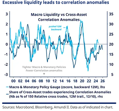
As a rule of thumb, excessively abundant liquidity is not favourable for alpha generation, as it leads to the misallocation of capital, with poorer fundamental discrimination, and correlation anomalies. Conversely, episodes of abnormally scarce liquidity tend to increase correlation among assets, overlooking idiosyncrasy, raising co-movement risk and portfolio volatility. Scarce liquidity also usually leads to lower asset price dispersion, limiting portfolio managers’ arbitrage opportunities. Overall, average-to-slightly-tight liquidity sets the optimal backdrop for active managers.

 

 

Changes in liquidity influence volatility regimes, which in turn affect risk premia and hedging strategies.

Additionally, liquidity affects the equity-bond correlation, especially at extreme levels: when liquidity is scarce, the equity-bond correlation tends to decline, enhancing the protective role of bonds.

 

 

Integrating liquidity in portfolio construction

Liquidity is a key macro variable alongside growth and inflation. This is illustrated on the following graph, which focuses on the US and shows the performance of a 60% Equity / 40% Bond allocation (“US 60/40 allocation”) under various macro combinations. The graph highlights that performance tends to decline and become unpredictable when liquidity tightens.

 

 

These macro variables collectively explain a significant portion of asset performance (about 2/3 over the long run), although their influence varies over time and across markets. Interconnected trends across global economies and transversal shocks also have a substantial impact on assets, beyond more idiosyncratic factors and FX exposure. Liquidity and its broad induced effects explain a significant share of recent performance, as shown in the below left graph, which highlights the contribution of these drivers to a US 60/40 allocation’s performance. 

 

 

In practice, factoring liquidity in portfolio construction can be implemented by:

• Determining each asset’s current exposure to liquidity. This sensitivity is not static: there are episodes when liquidity matters crucially, others when it matters less. 

  The right graph (on the previous page) shows the fluctuating exposure of the US 60-40 allocation to liquidity, based on models assessing the intensity, the stability and the reliability of the relationship across several time horizons (long, medium and short term): it shows that liquidity retains a significant influence today.

• Diversifying allocations according to liquidity profiles to enhance portfolio robustness.

• Adjusting portfolio weights based on liquidity regimes, which may influence cash levels and cyclical versus defensive allocations, and trading styles (tactical versus buy-and-hold).

• Stress testing portfolio performance under various liquidity stress scenarios to identify vulnerabilities.

• Considering reducing exposures when the liquidity signal seriously weakens (and vice versa).